Project a Stochastic Model Forward in Time
Source:R/projection_stochastic_model.R
projection_stochastic_model.RdRuns forward projections from the posterior draws of a fitted
abc_stochastic_model for a fixed number of time steps (default 30),
using region-specific states and parameter sets. Each simulation is seeded
for reproducibility and run in parallel.
If state doesn't exist e.g. "I" but has states "I_{age}" then will sum over all states first before plotting
take the difference of column(s) that match on state state. This is
useful for any cumulative columns e.g. INC and C by converted them into
the incidence and case incidence respectively
For cumulative state variables such as cases (e.g., C_[0,1)), this function
resets their values to 0 at a specified reference time (default is 0). This is
useful when wanting to compute cumulative changes from a particular time point
in a simulation or projection.
Usage
projection_stochastic_model(asm, project_time = 30, seed = 123)

add_projection_date(psm, start_date)

# S3 method for class 'projection_stochastic_model'
plot(x, ...)

plot_projections(projection, state)

plot_projection_samples(psm, state)

plot_projections_by_age_group(projection, state)

create_projection_quantiles(
  psm,
  probs = c(0.025, 0.25, 0.5, 0.75, 0.975),
  by_cols = c("time", "date")
)

projection_quantiles_by_age_group(
  psm,
  state,
  probs = c(0.025, 0.25, 0.5, 0.75, 0.975)
)

projection_by_age_group(psm, state)

create_age_group_column(psm, state, index_cols = c("date", "time"))

collapse_states(psm)

difference_of_states(psm, state)

reset_state(psm, state, reset_time = 0)
Arguments
- asm
An object of class
abc_stochastic_modelorscenario_stochastic_model.- project_time
Number of time steps to project forward. Defaults to
30.- seed
An integer used to seed the parallel simulations for reproducibility. Defaults to
123.- psm
An object of class
projection_stochastic_model, or a compatible data structure as accepted byget_projection_dataframe().- start_date
a date in yyyy-mm-dd format
- x
An object of class
projection_stochastic_model- ...
other arguments including
statestate to plot,"I"by default andtypeeither show individual trajectories "samples" or summarize "quantiles","quantiles"by default- projection
projection grouped using projection_quantiles_by_age_group
- state
A character string specifying the prefix of the cumulative state variable to reset (e.g.,
"C"to match columns like"C_[0,1)","C_[1,5)", etc.).- probs
vector of quantiles to plot
- by_cols
vector of columns to group by
- index_cols
columns to preserve defaults to
c("time","date")- reset_time
A numeric value indicating the time at which to reset the cumulative values back to zero. Defaults to 0.
Value
An object of class projection_stochastic_model, which is a list
with the following elements:
- model
The stochastic model used for simulation (of class
stochastic_model).- projection
A data frame with the projected simulations concatenated across posterior draws and days, including any parameter updates appended as columns.
An object of class projection_stochastic_model
A ggplot object.
A ggplot object.
A tibble() with columns by_cols, quantile, and quantile values per variable.
A tibble() with date, time, age_group, quantile, values.
tibble()
A tibble() in long format with age_group and the state column.
A tibble() with additional collapsed prefix columns
A tibble() with columns of differences per simulation trajectory
A tibble() with the same structure as the original projection data frame
Details
This function takes a fitted abc_stochastic_model, extracts the
posterior state and parameter sets, then runs simulations in parallel using
furrr. The model is updated with each posterior draw, run forward for a
fixed time frame, interpolated to daily resolution, and combined
into a single projection data frame.
Methods (by generic)
plot(projection_stochastic_model): Plot projections (quantiles or sample trajectories).
Functions
add_projection_date(): Add date to projection using astart_dateplot_projections(): Plot quantile bands (q2.5%, q25%, median, q75%, q97.5%) for a state.plot_projection_samples(): Plot individual sample trajectories, coloured by per-sample peak magnitude.plot_projections_by_age_group(): Faceted quantile plots by age group for a given state.create_projection_quantiles(): Compute per-time quantiles across simulations for all numeric columns.projection_quantiles_by_age_group(): Compute quantiles by age group for a state (e.g.,"C").projection_by_age_group(): Long-format projectiontibble()with anage_groupcolumn for a state prefix.create_age_group_column(): Create anage_groupcolumn by gathering state_AGE columns for a prefix state.collapse_states(): Sum age-stratified columns into their shared prefix (e.g.,C_[*]→C).difference_of_states(): Take first differences for all columns starting with a state prefix.reset_state(): Convert cumulative state variables back to zero at a reference time
Examples
# create stochastic model
reactions <- list(
infection_1 = list(
transition = c("I_1" = +1, "C" = +1),
rate = function(x,p,t){p$beta}
),
infection_2 = list(
transition = c("I_2" = +1, "C" = +1),
rate = function(x,p,t){0.5*p$beta}
)
)
example_scenario <- list(
params = list(beta = 0.1),
initial_states = list(I_1 = 0, I_2 = 0, C = 0),
sim_args = list(T = 10)
)
sm <- stochastic_model(reactions,example_scenario)
# project a scenario across a range of a single parameter value
parameters <- data.frame(beta = seq(0.1, 0.5, length.out = 10))
asm <- scenario_stochastic_model(sm, parameters = parameters)
psm <- projection_stochastic_model(asm)
# Add projection date
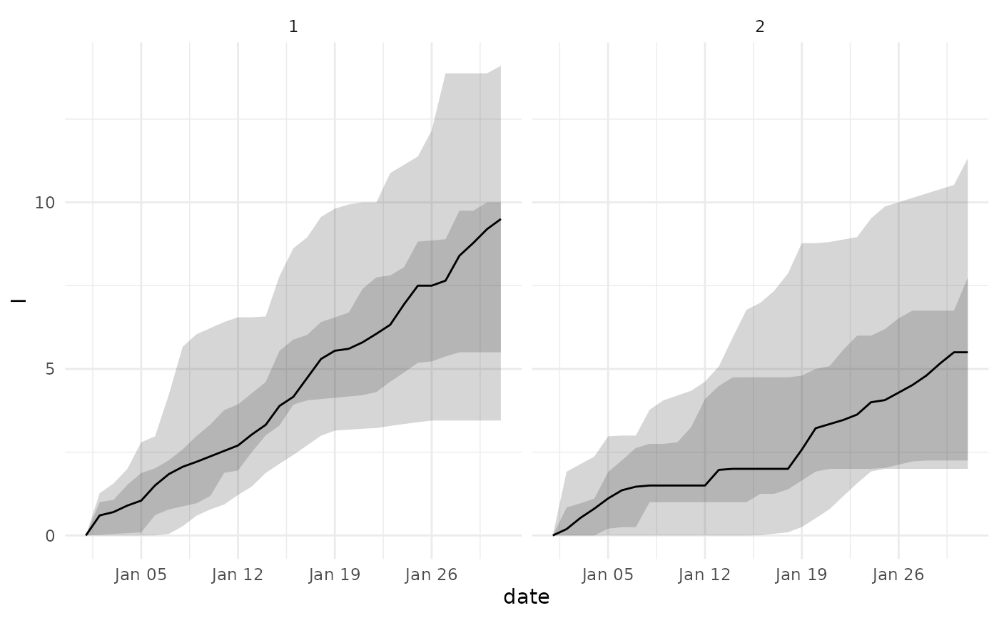
psm <- add_projection_date(psm, "2026-01-01")
# plots
plot(psm, state = "C", type = "quantiles")
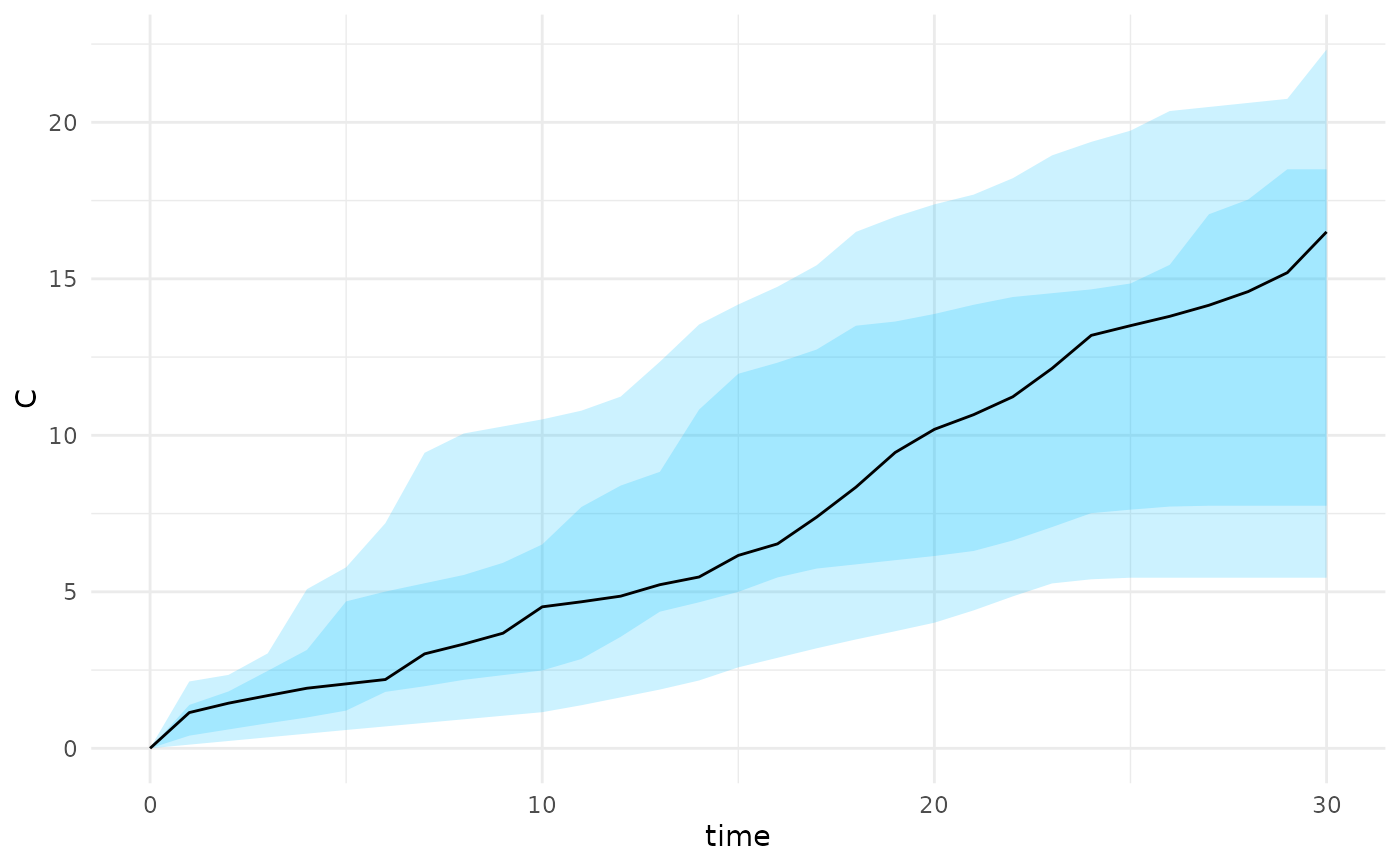
 plot_projections(psm, state = "C")
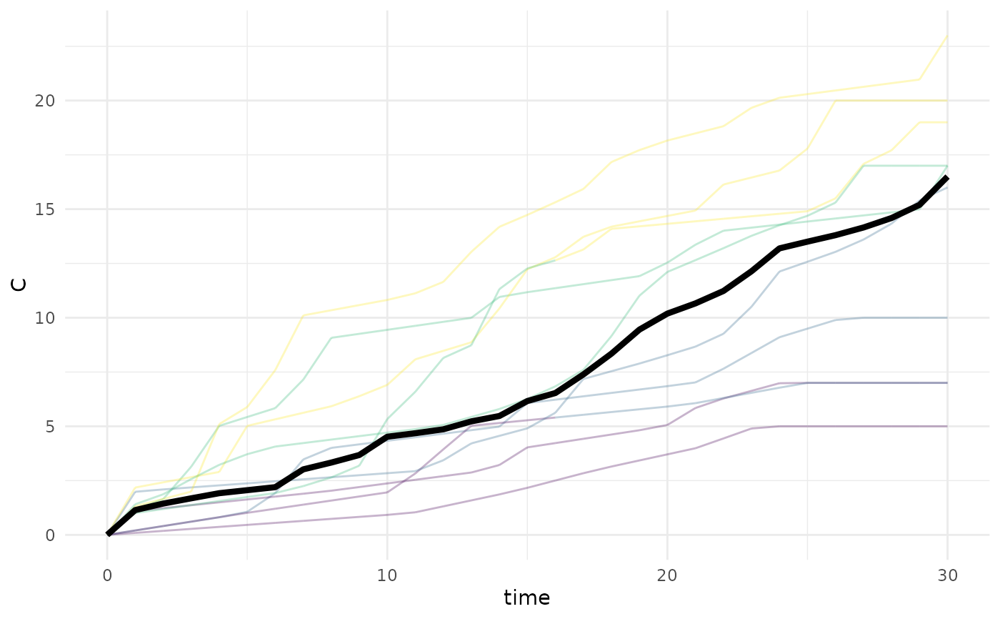
 plot_projection_samples(psm, state = "C")
#> Warning: Using `size` aesthetic for lines was deprecated in ggplot2 3.4.0.
#> ℹ Please use `linewidth` instead.
#> ℹ The deprecated feature was likely used in the brech package.
#> Please report the issue at <https://github.com/BCCDC-PHSA/brech/issues>.
plot_projection_samples(psm, state = "C")
#> Warning: Using `size` aesthetic for lines was deprecated in ggplot2 3.4.0.
#> ℹ Please use `linewidth` instead.
#> ℹ The deprecated feature was likely used in the brech package.
#> Please report the issue at <https://github.com/BCCDC-PHSA/brech/issues>.
 # plots by age group
projection <- projection_quantiles_by_age_group(psm, "I")
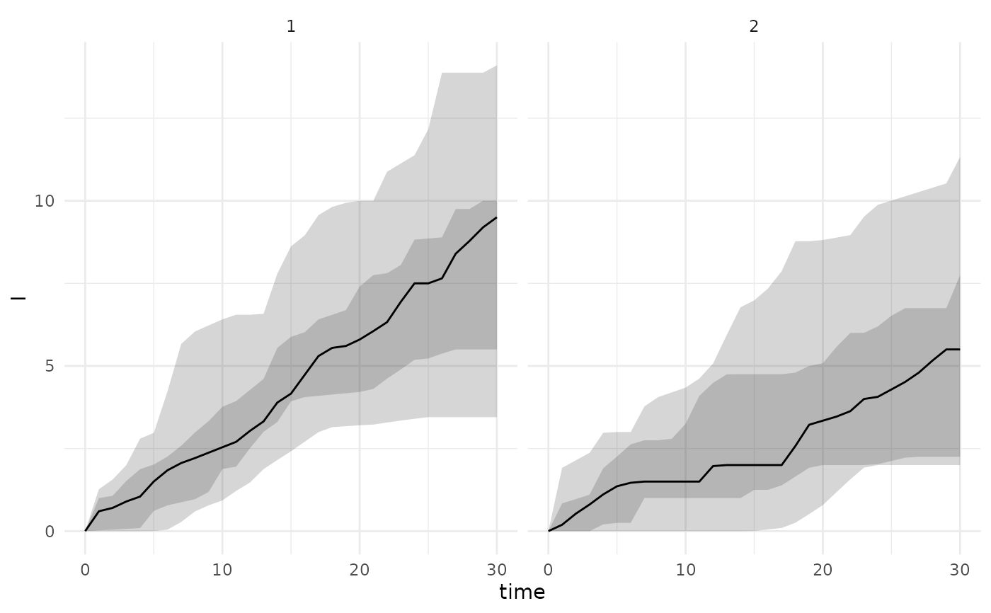
plot_projections_by_age_group(projection,"I")
# plots by age group
projection <- projection_quantiles_by_age_group(psm, "I")
plot_projections_by_age_group(projection,"I")
 # projection transformation and summaries
create_projection_quantiles(psm)
#> # A tibble: 155 × 7
#> time date I_1 I_2 C beta quantile
#> <int> <date> <dbl> <dbl> <dbl> <dbl> <dbl>
#> 1 0 2026-01-01 0 0 0 0.11 0.025
#> 2 0 2026-01-01 0 0 0 0.2 0.25
#> 3 0 2026-01-01 0 0 0 0.3 0.5
#> 4 0 2026-01-01 0 0 0 0.4 0.75
#> 5 0 2026-01-01 0 0 0 0.49 0.975
#> 6 1 2026-01-02 0 0 0.117 0.11 0.025
#> 7 1 2026-01-02 0.0230 0 0.404 0.2 0.25
#> 8 1 2026-01-02 0.602 0.193 1.14 0.3 0.5
#> 9 1 2026-01-02 1 0.841 1.39 0.4 0.75
#> 10 1 2026-01-02 1.27 1.92 2.14 0.49 0.975
#> # ℹ 145 more rows
projection_quantiles_by_age_group(psm, state = "I")
#> # A tibble: 310 × 5
#> date time age_group quantile values
#> <date> <int> <chr> <dbl> <dbl>
#> 1 2026-01-01 0 1 0.025 0
#> 2 2026-01-01 0 1 0.25 0
#> 3 2026-01-01 0 1 0.5 0
#> 4 2026-01-01 0 1 0.75 0
#> 5 2026-01-01 0 1 0.975 0
#> 6 2026-01-01 0 2 0.025 0
#> 7 2026-01-01 0 2 0.25 0
#> 8 2026-01-01 0 2 0.5 0
#> 9 2026-01-01 0 2 0.75 0
#> 10 2026-01-01 0 2 0.975 0
#> # ℹ 300 more rows
projection_by_age_group(psm, state = "I")
#> # A tibble: 620 × 4
#> date time age_group I
#> <date> <int> <chr> <dbl>
#> 1 2026-01-01 0 1 0
#> 2 2026-01-01 0 2 0
#> 3 2026-01-02 1 1 0.0921
#> 4 2026-01-02 1 2 0
#> 5 2026-01-03 2 1 0.184
#> 6 2026-01-03 2 2 0
#> 7 2026-01-04 3 1 0.276
#> 8 2026-01-04 3 2 0
#> 9 2026-01-05 4 1 0.369
#> 10 2026-01-05 4 2 0
#> # ℹ 610 more rows
create_age_group_column(psm, state = "I")
#> # A tibble: 620 × 4
#> date time age_group I
#> <date> <int> <chr> <dbl>
#> 1 2026-01-01 0 1 0
#> 2 2026-01-01 0 2 0
#> 3 2026-01-02 1 1 0.0921
#> 4 2026-01-02 1 2 0
#> 5 2026-01-03 2 1 0.184
#> 6 2026-01-03 2 2 0
#> 7 2026-01-04 3 1 0.276
#> 8 2026-01-04 3 2 0
#> 9 2026-01-05 4 1 0.369
#> 10 2026-01-05 4 2 0
#> # ℹ 610 more rows
collapse_states(psm)
#> # A tibble: 310 × 7
#> time I_1 I_2 C beta date I
#> <int> <dbl> <dbl> <dbl> <dbl> <date> <dbl>
#> 1 0 0 0 0 0.1 2026-01-01 0
#> 2 1 0.0921 0 0.0921 0.1 2026-01-02 0.0921
#> 3 2 0.184 0 0.184 0.1 2026-01-03 0.184
#> 4 3 0.276 0 0.276 0.1 2026-01-04 0.276
#> 5 4 0.369 0 0.369 0.1 2026-01-05 0.369
#> 6 5 0.461 0 0.461 0.1 2026-01-06 0.461
#> 7 6 0.553 0 0.553 0.1 2026-01-07 0.553
#> 8 7 0.645 0 0.645 0.1 2026-01-08 0.645
#> 9 8 0.737 0 0.737 0.1 2026-01-09 0.737
#> 10 9 0.829 0 0.829 0.1 2026-01-10 0.829
#> # ℹ 300 more rows
difference_of_states(psm, state = "C")
#> # A tibble: 310 × 7
#> time I_1 I_2 C beta date sim_id
#> <int> <dbl> <dbl> <dbl> <dbl> <date> <int>
#> 1 0 0 0 0 0.1 2026-01-01 1
#> 2 1 0.0921 0 0.0921 0.1 2026-01-02 1
#> 3 2 0.184 0 0.184 0.1 2026-01-03 1
#> 4 3 0.276 0 0.276 0.1 2026-01-04 1
#> 5 4 0.369 0 0.369 0.1 2026-01-05 1
#> 6 5 0.461 0 0.461 0.1 2026-01-06 1
#> 7 6 0.553 0 0.553 0.1 2026-01-07 1
#> 8 7 0.645 0 0.645 0.1 2026-01-08 1
#> 9 8 0.737 0 0.737 0.1 2026-01-09 1
#> 10 9 0.829 0 0.829 0.1 2026-01-10 1
#> # ℹ 300 more rows
# Reset cumulative cases to 0 at time 5
reset_state(psm, state = "C", reset_time = 5)
#> # A tibble: 310 × 7
#> time I_1 I_2 C beta date sim_id
#> <int> <dbl> <dbl> <dbl> <dbl> <date> <int>
#> 1 0 0 0 0 0.1 2026-01-01 1
#> 2 1 0.0921 0 0.0921 0.1 2026-01-02 1
#> 3 2 0.184 0 0.184 0.1 2026-01-03 1
#> 4 3 0.276 0 0.276 0.1 2026-01-04 1
#> 5 4 0.369 0 0.369 0.1 2026-01-05 1
#> 6 5 0.461 0 0.461 0.1 2026-01-06 1
#> 7 6 0.553 0 0.553 0.1 2026-01-07 1
#> 8 7 0.645 0 0.645 0.1 2026-01-08 1
#> 9 8 0.737 0 0.737 0.1 2026-01-09 1
#> 10 9 0.829 0 0.829 0.1 2026-01-10 1
#> # ℹ 300 more rows
# projection transformation and summaries
create_projection_quantiles(psm)
#> # A tibble: 155 × 7
#> time date I_1 I_2 C beta quantile
#> <int> <date> <dbl> <dbl> <dbl> <dbl> <dbl>
#> 1 0 2026-01-01 0 0 0 0.11 0.025
#> 2 0 2026-01-01 0 0 0 0.2 0.25
#> 3 0 2026-01-01 0 0 0 0.3 0.5
#> 4 0 2026-01-01 0 0 0 0.4 0.75
#> 5 0 2026-01-01 0 0 0 0.49 0.975
#> 6 1 2026-01-02 0 0 0.117 0.11 0.025
#> 7 1 2026-01-02 0.0230 0 0.404 0.2 0.25
#> 8 1 2026-01-02 0.602 0.193 1.14 0.3 0.5
#> 9 1 2026-01-02 1 0.841 1.39 0.4 0.75
#> 10 1 2026-01-02 1.27 1.92 2.14 0.49 0.975
#> # ℹ 145 more rows
projection_quantiles_by_age_group(psm, state = "I")
#> # A tibble: 310 × 5
#> date time age_group quantile values
#> <date> <int> <chr> <dbl> <dbl>
#> 1 2026-01-01 0 1 0.025 0
#> 2 2026-01-01 0 1 0.25 0
#> 3 2026-01-01 0 1 0.5 0
#> 4 2026-01-01 0 1 0.75 0
#> 5 2026-01-01 0 1 0.975 0
#> 6 2026-01-01 0 2 0.025 0
#> 7 2026-01-01 0 2 0.25 0
#> 8 2026-01-01 0 2 0.5 0
#> 9 2026-01-01 0 2 0.75 0
#> 10 2026-01-01 0 2 0.975 0
#> # ℹ 300 more rows
projection_by_age_group(psm, state = "I")
#> # A tibble: 620 × 4
#> date time age_group I
#> <date> <int> <chr> <dbl>
#> 1 2026-01-01 0 1 0
#> 2 2026-01-01 0 2 0
#> 3 2026-01-02 1 1 0.0921
#> 4 2026-01-02 1 2 0
#> 5 2026-01-03 2 1 0.184
#> 6 2026-01-03 2 2 0
#> 7 2026-01-04 3 1 0.276
#> 8 2026-01-04 3 2 0
#> 9 2026-01-05 4 1 0.369
#> 10 2026-01-05 4 2 0
#> # ℹ 610 more rows
create_age_group_column(psm, state = "I")
#> # A tibble: 620 × 4
#> date time age_group I
#> <date> <int> <chr> <dbl>
#> 1 2026-01-01 0 1 0
#> 2 2026-01-01 0 2 0
#> 3 2026-01-02 1 1 0.0921
#> 4 2026-01-02 1 2 0
#> 5 2026-01-03 2 1 0.184
#> 6 2026-01-03 2 2 0
#> 7 2026-01-04 3 1 0.276
#> 8 2026-01-04 3 2 0
#> 9 2026-01-05 4 1 0.369
#> 10 2026-01-05 4 2 0
#> # ℹ 610 more rows
collapse_states(psm)
#> # A tibble: 310 × 7
#> time I_1 I_2 C beta date I
#> <int> <dbl> <dbl> <dbl> <dbl> <date> <dbl>
#> 1 0 0 0 0 0.1 2026-01-01 0
#> 2 1 0.0921 0 0.0921 0.1 2026-01-02 0.0921
#> 3 2 0.184 0 0.184 0.1 2026-01-03 0.184
#> 4 3 0.276 0 0.276 0.1 2026-01-04 0.276
#> 5 4 0.369 0 0.369 0.1 2026-01-05 0.369
#> 6 5 0.461 0 0.461 0.1 2026-01-06 0.461
#> 7 6 0.553 0 0.553 0.1 2026-01-07 0.553
#> 8 7 0.645 0 0.645 0.1 2026-01-08 0.645
#> 9 8 0.737 0 0.737 0.1 2026-01-09 0.737
#> 10 9 0.829 0 0.829 0.1 2026-01-10 0.829
#> # ℹ 300 more rows
difference_of_states(psm, state = "C")
#> # A tibble: 310 × 7
#> time I_1 I_2 C beta date sim_id
#> <int> <dbl> <dbl> <dbl> <dbl> <date> <int>
#> 1 0 0 0 0 0.1 2026-01-01 1
#> 2 1 0.0921 0 0.0921 0.1 2026-01-02 1
#> 3 2 0.184 0 0.184 0.1 2026-01-03 1
#> 4 3 0.276 0 0.276 0.1 2026-01-04 1
#> 5 4 0.369 0 0.369 0.1 2026-01-05 1
#> 6 5 0.461 0 0.461 0.1 2026-01-06 1
#> 7 6 0.553 0 0.553 0.1 2026-01-07 1
#> 8 7 0.645 0 0.645 0.1 2026-01-08 1
#> 9 8 0.737 0 0.737 0.1 2026-01-09 1
#> 10 9 0.829 0 0.829 0.1 2026-01-10 1
#> # ℹ 300 more rows
# Reset cumulative cases to 0 at time 5
reset_state(psm, state = "C", reset_time = 5)
#> # A tibble: 310 × 7
#> time I_1 I_2 C beta date sim_id
#> <int> <dbl> <dbl> <dbl> <dbl> <date> <int>
#> 1 0 0 0 0 0.1 2026-01-01 1
#> 2 1 0.0921 0 0.0921 0.1 2026-01-02 1
#> 3 2 0.184 0 0.184 0.1 2026-01-03 1
#> 4 3 0.276 0 0.276 0.1 2026-01-04 1
#> 5 4 0.369 0 0.369 0.1 2026-01-05 1
#> 6 5 0.461 0 0.461 0.1 2026-01-06 1
#> 7 6 0.553 0 0.553 0.1 2026-01-07 1
#> 8 7 0.645 0 0.645 0.1 2026-01-08 1
#> 9 8 0.737 0 0.737 0.1 2026-01-09 1
#> 10 9 0.829 0 0.829 0.1 2026-01-10 1
#> # ℹ 300 more rows