library(ggplot2)
library(dplyr)
#>
#> Attaching package: 'dplyr'
#> The following objects are masked from 'package:stats':
#>
#>     filter, lag
#> The following objects are masked from 'package:base':
#>
#>     intersect, setdiff, setequal, union
library(tidyr)
library(brech)
set.seed(42)
Introduction
To create a model simulation we construct an R S3 object using the
stochastic_model class. This expects a list of reactions
including the transitions: the impact on the population and
rate: the rate at which the event takes place. e.g. the
first reaction represents an infection event that occurs at rate
where
is the population of susceptible,
is the population of infected and
is the population infectivity.
reactions <- list(
  infection = list(
    transition = c(S = -1, E = +1),
    rate = function(x, p, t) p$beta * x["S"] * x["I"]
  ),
  incubation = list(
    transition = c(E = -1, I = +1),
    rate = function(x, p, t) p$theta * x["E"]
  ),
  recovery = list(
    transition = c(I = -1, R = +1),
    rate = function(x, p, t) p$gamma * x["I"]
  ),
  case_detection = list(
    transition = c(C = +1),
    rate = function(x, p, t) p$case_rate * x["I"]
  ),
  vaccinate = list(
    transition = c(V = +1, S = -1),
    rate = function(x, p, t) 0 * x["S"]
  )
)
sim_scenario <- load_model_params() |>
  vaccinate_initial_conditions(0.8) |>
  update_parameters(beta=0.02)

sm <- stochastic_model(reactions,sim_scenario)
sm
#> Stochastic Model
#> ==================
#>
#> Initial Values:
#>   S : 200  V : 799  E : 0
#>   I : 1  R : 0  C : 0
#>   D : 0
#> Parameters:
#>   r_0 : 25  latent_period : 11  infectious_period : 8
#>   ascertainment_delay : 2.5  case_delay : 3  theta : 0.0909
#>   gamma : 0.125  case_rate : 0.333  beta : 0.02
#>   N : 1000
#> Simulation arguments:
#>   T : 10
#> Reactions:
#>  - infection:
#>    Transition: [S -1, E +1]
#>  - incubation:
#>    Transition: [E -1, I +1]
#>  - recovery:
#>    Transition: [I -1, R +1]
#>  - case_detection:
#>    Transition: [C +1]
#>  - vaccinate:
#>    Transition: [V +1, S -1]
#>
To run with default settings, just use the run_sim
function
Model fitting
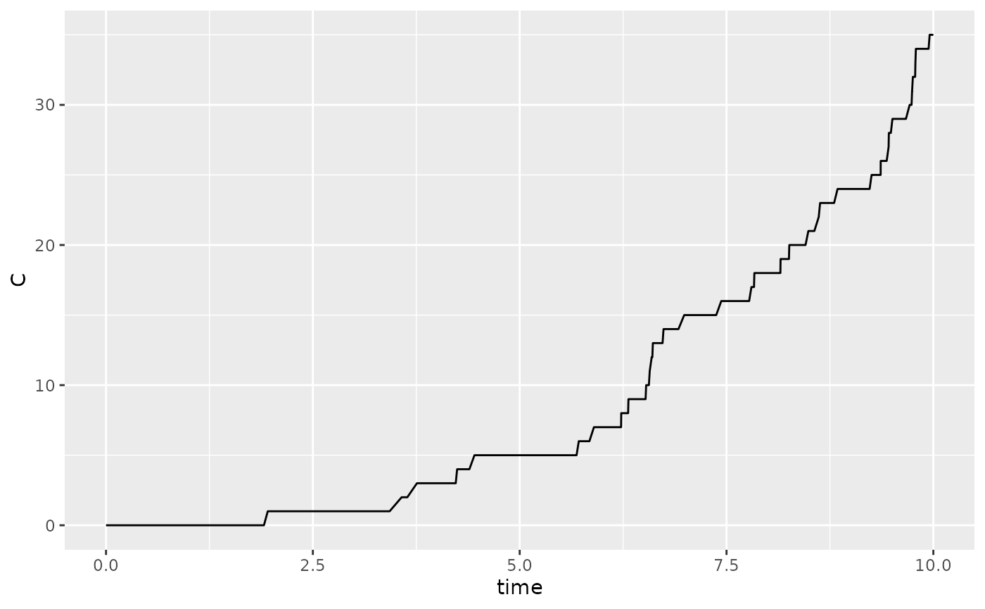
Approximate Bayesian Computation (ABC) is used to perform model fitting. This is done by defining a summary statistic and then running the summary statistic on the data. We will use the data above as an example and create a summary statistic for the cumulative number of cases after 10 days.
We then draw priors from a defined distribution for each parameter to
be fit. In the example below the parameter beta if fit to
the cumulative number of cases.
# generate summary statistics from run
# These are the number of cases on a given day
daily_cases <- sum(get_daily_cases(r)$daily_incidence)

# simulate from prior
priors <- tibble("beta" = pmax(0,rnorm(200,mean=0.1,sd=0.1)))

# statistical summary of simulation
stat_func <- function(m){
  #' get total cases
  m |>
    get_daily_cases() |>
    dplyr::summarise(total_cases=sum(daily_incidence))
}

res <- abc_stochastic_model(sm,priors,daily_cases,stat_func)

plot(res,param = "beta")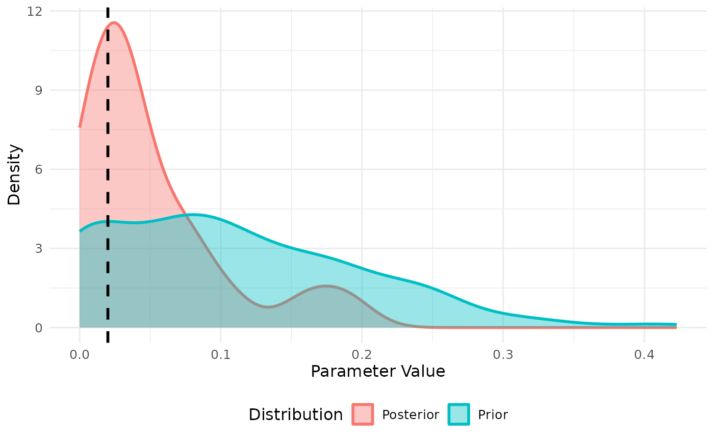
We can similarly fit to daily cases. Note that we need to exclude the first few days in the simulation where the variance in case incidence is too low. Fitting the incidence appears to improve the model fit with this small sample.
# simulate from prior
priors <- tibble("beta" = pmax(0,rnorm(200,mean=0.1,sd=0.1)))

# statistical summary of simulation
stat_func <- function(m){
  #' get total cases
  m |>
    get_daily_cases() |>
    filter(day > 3) |>
    pivot_wider(names_from = "day",values_from="daily_incidence",
                names_prefix = "day_")
}

daily_cases <- stat_func(r)

res <- abc_stochastic_model(sm,priors,daily_cases,stat_func)

plot(res, param = "beta")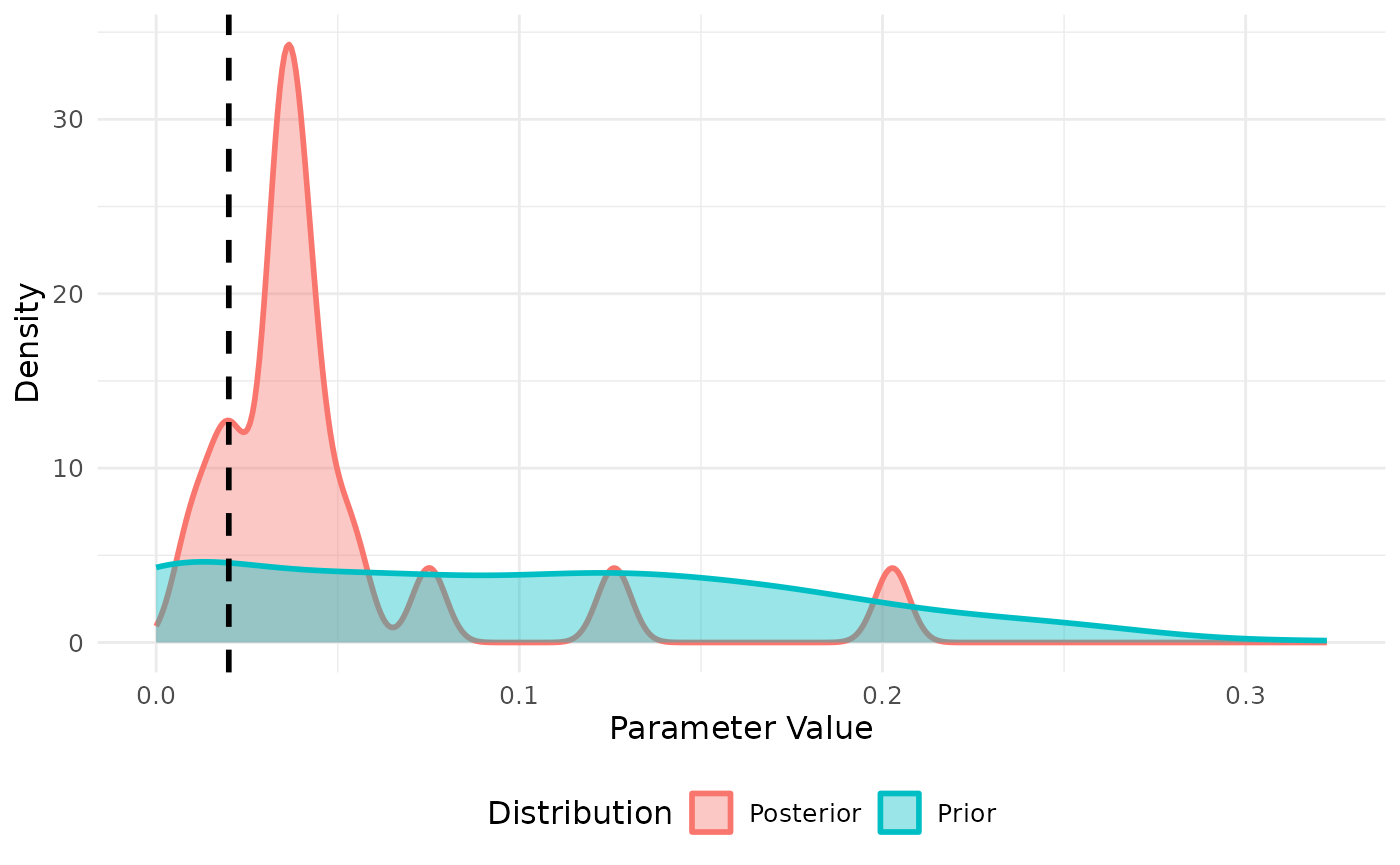
The fit also provides the final state of each simulation from the posterior which we can compare to our fitted data
data.frame(r) |>
  filter(time == max(time)) |>
  dplyr::select(-time) |>
  mutate(type = "true value") |>
  bind_rows(
    mutate(res$state,type="posterior")
  ) |>
  pivot_longer(-type,names_to = "state", values_to = "value") |>
  ggplot(aes(x=state,y=value,color=type)) +
  geom_jitter(alpha=0.5)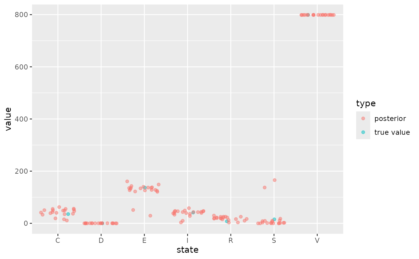
Scenario projection
We can then perform projections using a
abc_stochastic_model object. The projection will sample
over the final state of the model in the posterior as well as any
associated parameters and inherit other parameters from the underlying
stochastic_model class. We project forward in time using
the projection_stochastic_model function which also comes
with default plotting behaviour.
projections <- projection_stochastic_model(res)
plot(projections, state = "I")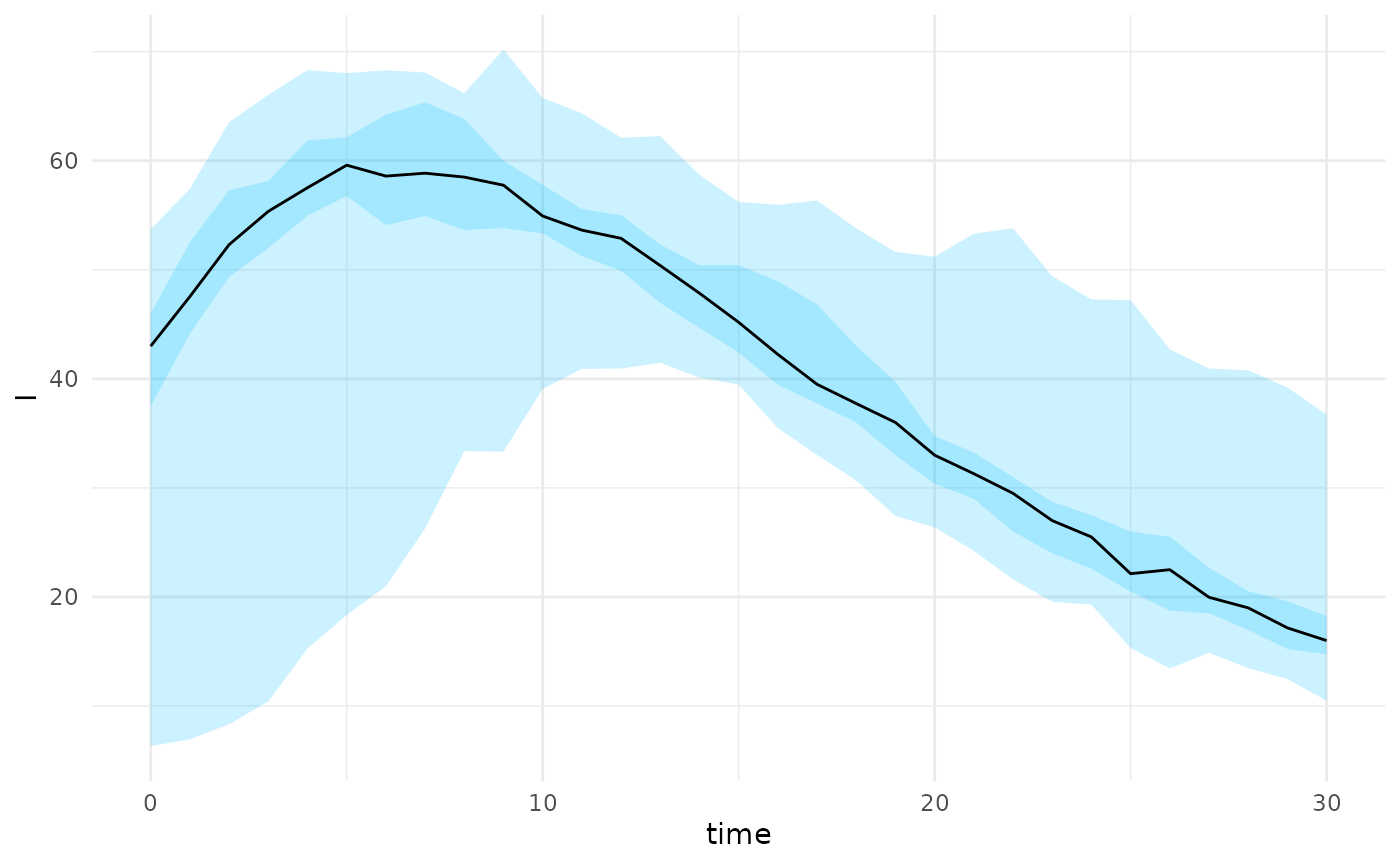
plot(projections, state = "C")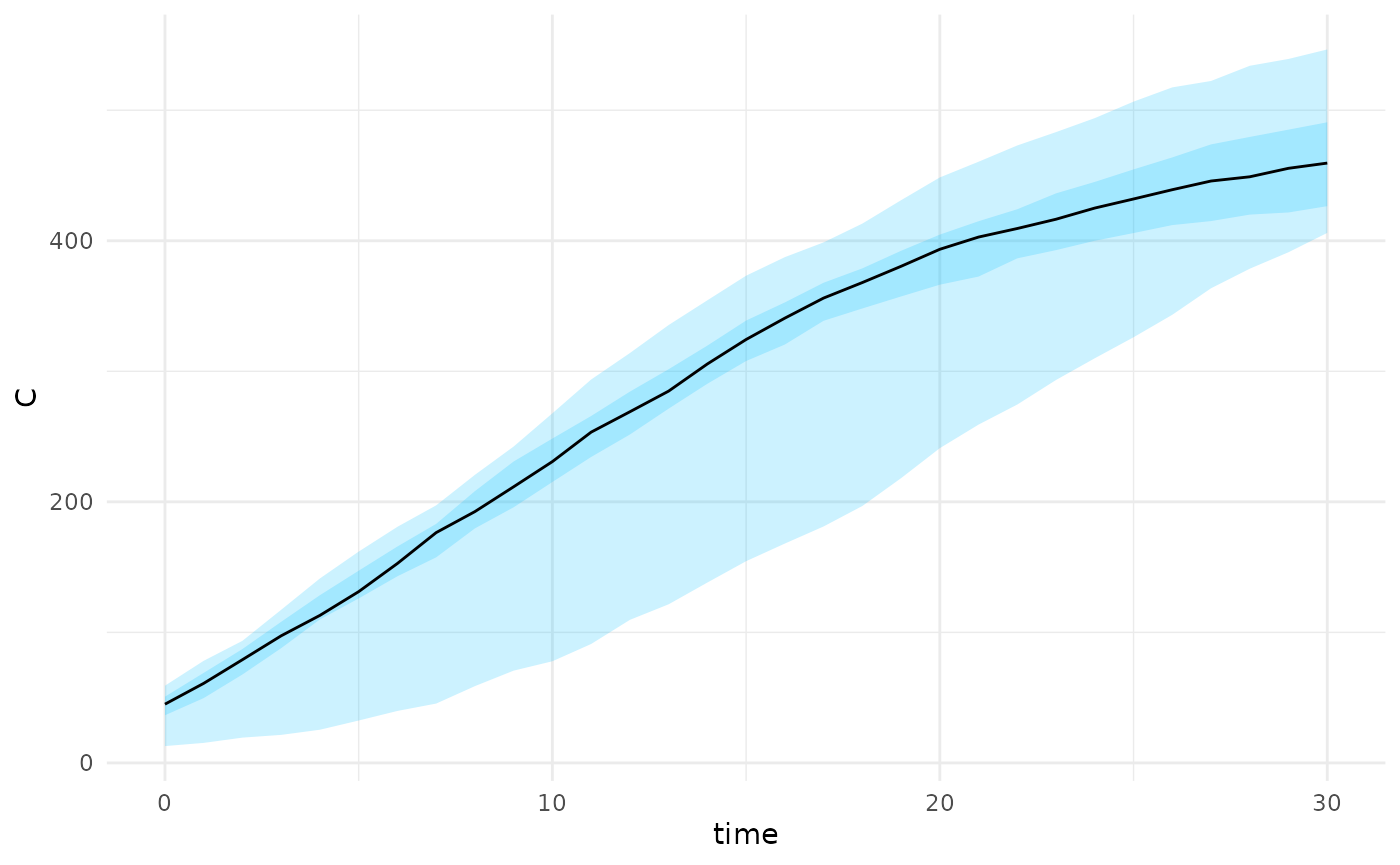
The projection_stochastic_model function can also
incorporate scenarios directly without the need for model fitting. This
is useful if there is a need to project under different scenarios where
there is no current data to inform the model fit. Under this scenario we
draw from a defined distribution of
parameters
parameters <- tibble("beta" = runif(200,min=0.08,max=0.12))
scenarios <- scenario_stochastic_model(sm,parameters)
projections <- projection_stochastic_model(scenarios)
plot(projections, state = "I")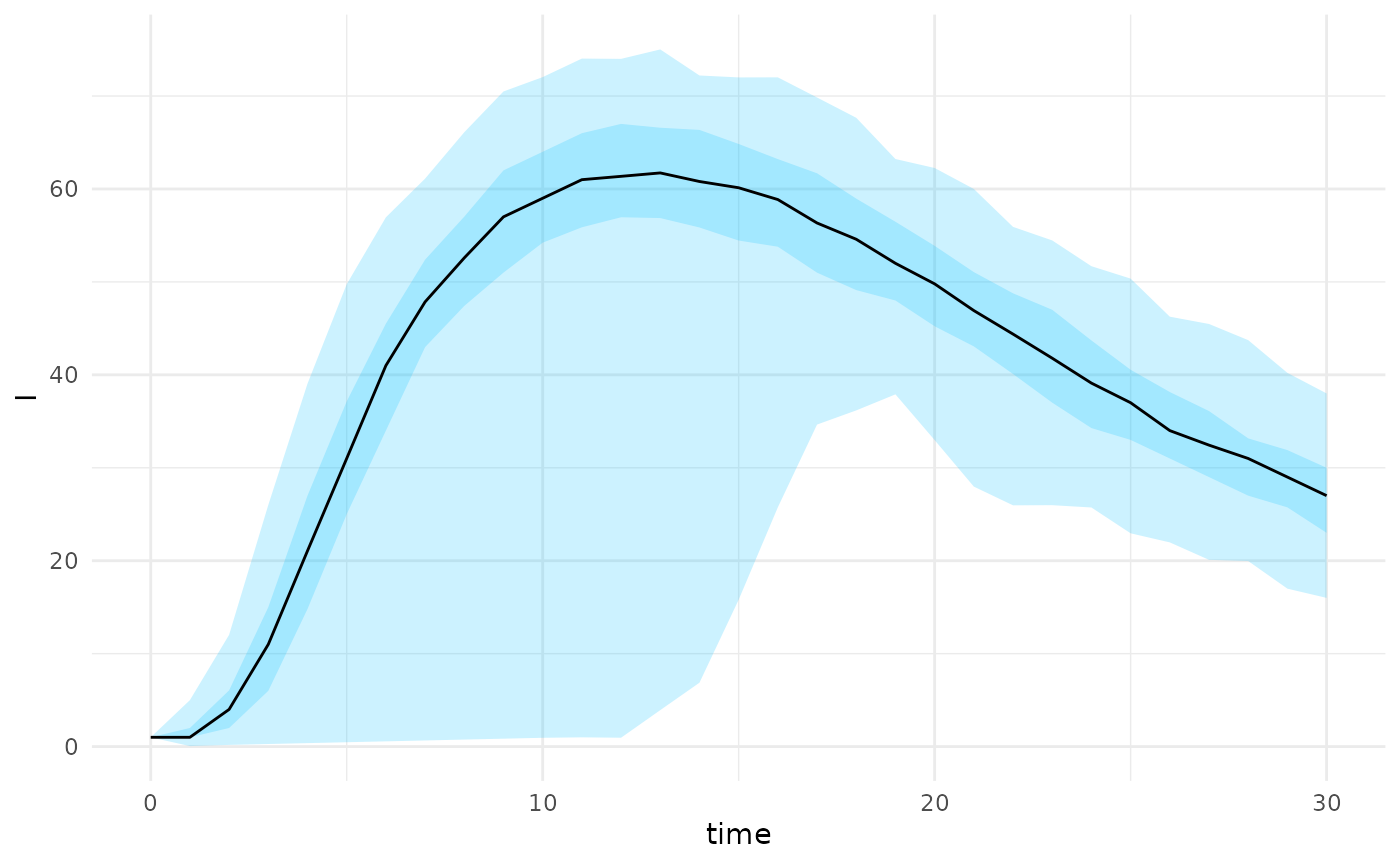
A flow chart of the dependency between defined S3 classes in the
package is provided below. The base class is
stochastic_model which defines the model events, rates,
parameters and initial states. A summary of the object can
be provided and a simulation can be drawn from the model using the
function run_sim(). Model fitting can be performed using
the abc_stochastic_model or alternatively a scenario can be
generated using the scenario_stochastic_model class.
Finally a projection can be generated from either a scenario or model
fit using projection_stochastic_model.
flowchart TD
  M("load_parameters()") --> A
  R("reactions") --> A
  A[stochastic_model] --> B[abc_stochastic_model]
  A --> C[scenario_stochastic_model]
  B --> D[projection_stochastic_model]
  C --> D
Age-structured model
For an age structured model we need to set-up reactions for each age-group. This can be done explicitly as above, however would quickly become cumbersome for a large number of age-groups. Instead we can construct this by looping over age groups and defining each of the reactions e.g. “infection” and “recovery”. This requires that the rates functions are built inside a function factory to ensure that the correct age-parameters are provided to each function. For more information see this chapter.
First we construct a simple contact age contact matrix with two age groups,
age_groups <- c("<18", "18+")
contact_matrix <- matrix(c(20,5,5,10), nrow = 2)
rownames(contact_matrix) <- age_groups
colnames(contact_matrix) <- age_groups
print(contact_matrix)
#>     <18 18+
#> <18  20   5
#> 18+   5  10
Next we use the age_groups and
contact_matrix to populate the reactions list.
To illustrate the code below provides a simple age-structured SIR model.
We encapsulate this inside a function to ensure that variables such as
age_groups can be referenced later.
create_custom_reactions <- function(contact_matrix){
  age_groups <- colnames(contact_matrix)
  reactions <- list()
  for (i in seq_along(age_groups)){
        age_group <- age_groups[i]
        ###########################
        #  infection transitions  #
        ###########################
        transition <- function() {
          trans <- c()
          trans[paste0("S_",age_group)] <- -1
          trans[paste0("I_",age_group)] <- +1
          trans
        }
        rate <-
          function(i,age_group){
            force(i)
            force(age_group)
            function(x, p, t) {
              I <- x[paste0("I_", age_groups)]
              S <- x[paste0("S_", age_group)]
              lambda <- p$beta * S * sum(contact_matrix[,i] * (I / p$N))
              lambda
            }
          }
        reactions[[paste0("infection_",age_group)]] <- list(
          "transition"=transition(),
          "rate" = rate(i,age_group)
        )
        ##############################
        #    recovery transitions    #
        ##############################
        transition <- function() {
          trans <- c()
          trans[paste0("I_",age_group)] <- -1
          trans[paste0("R_",age_group)] <- + 1
          trans
        }
        rate <-
        function(age_group){
          force(age_group)
          function(x, p, t) {
            I <- x[paste0("I_", age_group)]
            p$gamma * I
          }
        }
        reactions[[paste0("recovery_",age_group)]] <- list(
          "transition"=transition(),
          "rate" = rate(age_group)
        )

  }
  return(reactions)
}

reactions <- create_custom_reactions(contact_matrix)
We then apply these reactions to construct a
stochastic_model object. We use the function
create_age_initial_conditions to convert the initial
conditions from a vector format to the format required for the
object.
age_scenario <- list(
  params = list(beta = 0.5, gamma = 0.2, N = 1000),
  initial_states = list(
    S = c(200, 800),
    V = c(0, 0),
    I = c(1, 0),
    R = c(0, 0)
    ),
  sim_args = list(T = 10)
)

age_scenario <- age_scenario |>
  create_age_initial_conditions(age_groups)


sm <- stochastic_model(reactions,age_scenario)
print(sm)
#> Stochastic Model
#> ==================
#>
#> Initial Values:
#>   S_<18 : 200  S_18+ : 800  V_<18 : 0
#>   V_18+ : 0  I_<18 : 1  I_18+ : 0
#>   R_<18 : 0  R_18+ : 0
#> Parameters:
#>   beta : 0.5  gamma : 0.2  N : 1000
#>
#> Simulation arguments:
#>   T : 10
#> Reactions:
#>  - infection_<18:
#>    Transition: [S_<18 -1, I_<18 +1]
#>  - recovery_<18:
#>    Transition: [I_<18 -1, R_<18 +1]
#>  - infection_18+:
#>    Transition: [S_18+ -1, I_18+ +1]
#>  - recovery_18+:
#>    Transition: [I_18+ -1, R_18+ +1]
#>
As before we can run this simulation and plot
r <- sm |>
    run_sim() |>
    as.data.frame() |>
    tidyr::pivot_longer(
      cols = tidyselect::starts_with("I_"),
      names_to = "age_group",
      names_prefix = "I_",
      values_to = "I"
    )
r |> ggplot(aes(x=time,y=I, color= age_group)) + geom_line()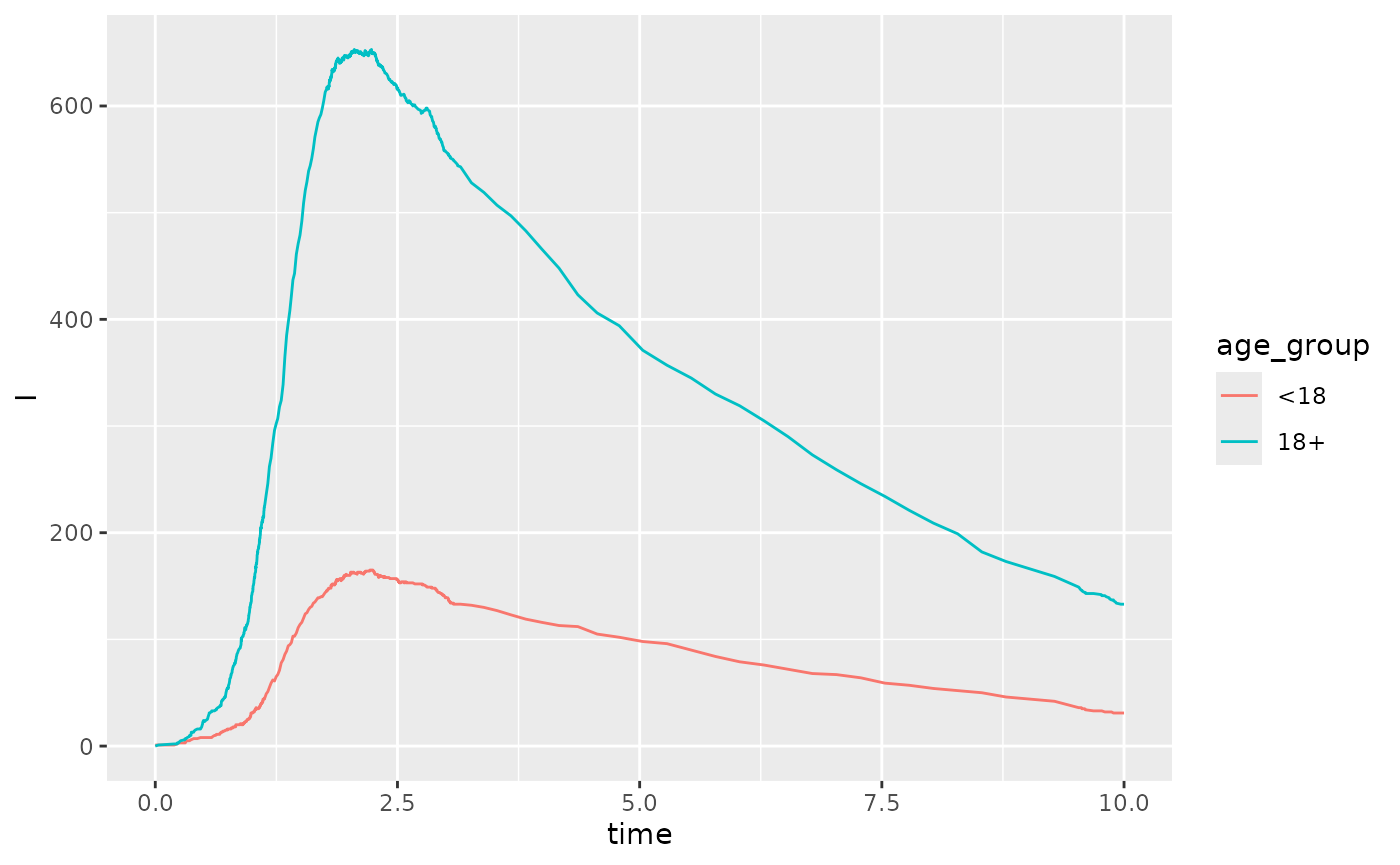
We can also vaccinate the initial population by age group. In the example below we imagine that the <18 age group is 10% vaccinated and the 18+ age group is 90% vaccinated. Notice that the initial values are now updated.
sm |> vaccinate_initial_conditions(c("<18"=0.1,"18+"=0.9))
#> Stochastic Model
#> ==================
#>
#> Initial Values:
#>   S_<18 : 180  S_18+ : 80  V_<18 : 20
#>   V_18+ : 720  I_<18 : 1  I_18+ : 0
#>   R_<18 : 0  R_18+ : 0
#> Parameters:
#>   beta : 0.5  gamma : 0.2  N : 1000
#>
#> Simulation arguments:
#>   T : 10
#> Reactions:
#>  - infection_<18:
#>    Transition: [S_<18 -1, I_<18 +1]
#>  - recovery_<18:
#>    Transition: [I_<18 -1, R_<18 +1]
#>  - infection_18+:
#>    Transition: [S_18+ -1, I_18+ +1]
#>  - recovery_18+:
#>    Transition: [I_18+ -1, R_18+ +1]
#>
We can similarly generate projections using the
scenario_stochastic_model object,
parameters <- tibble("beta" = runif(200,min=0.08,max=0.12))
scenarios <- scenario_stochastic_model(sm,parameters)
projections <- projection_stochastic_model(scenarios)
plot(projections, state = "I")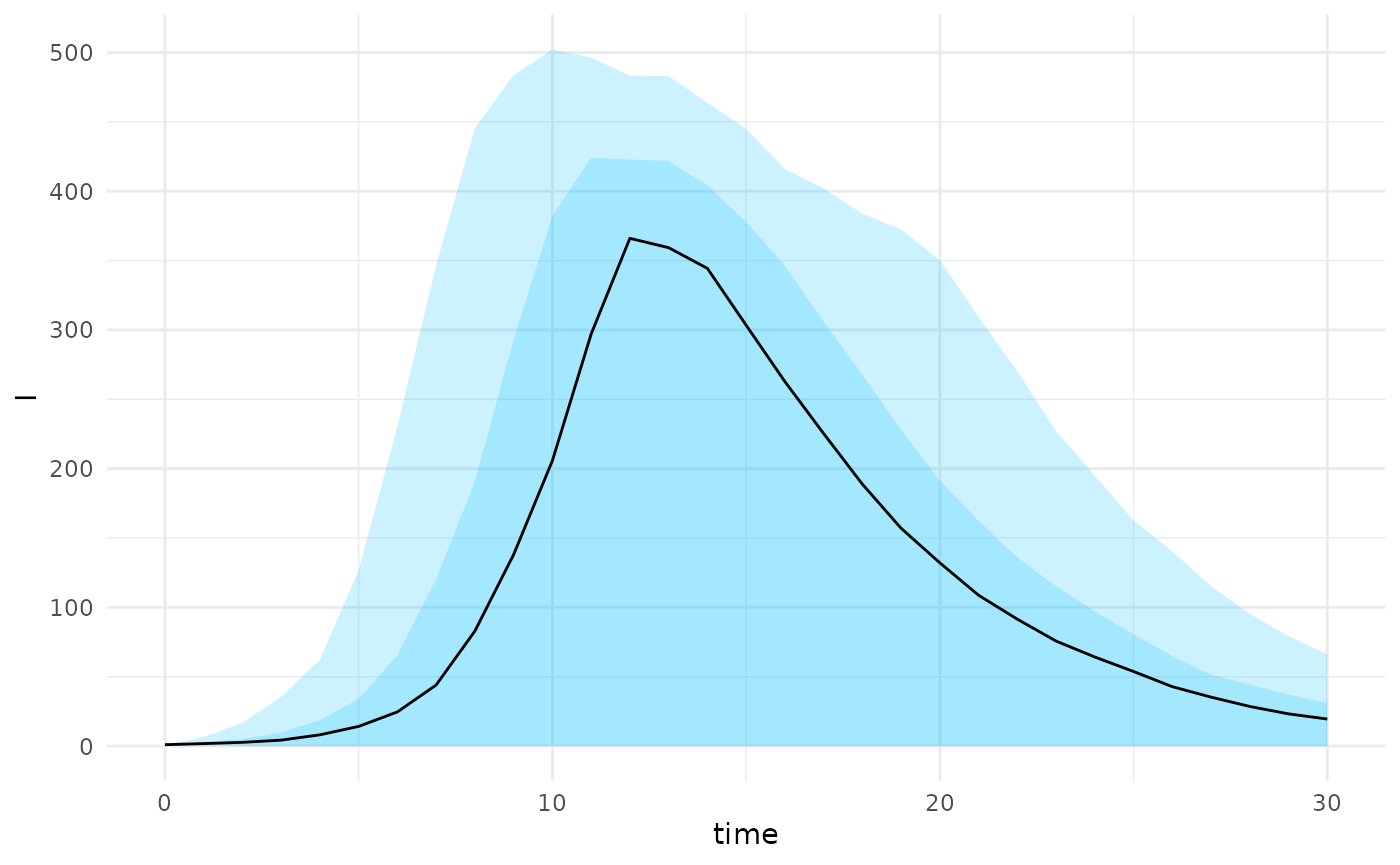
A series of helper functions can also be used to construct quantiles
and plot summaries from an age-structured model as long as the states
are named in the format {model_state}_{age_group}.
projections |>
  projection_quantiles_by_age_group("I") |>
  plot_projections_by_age_group("I")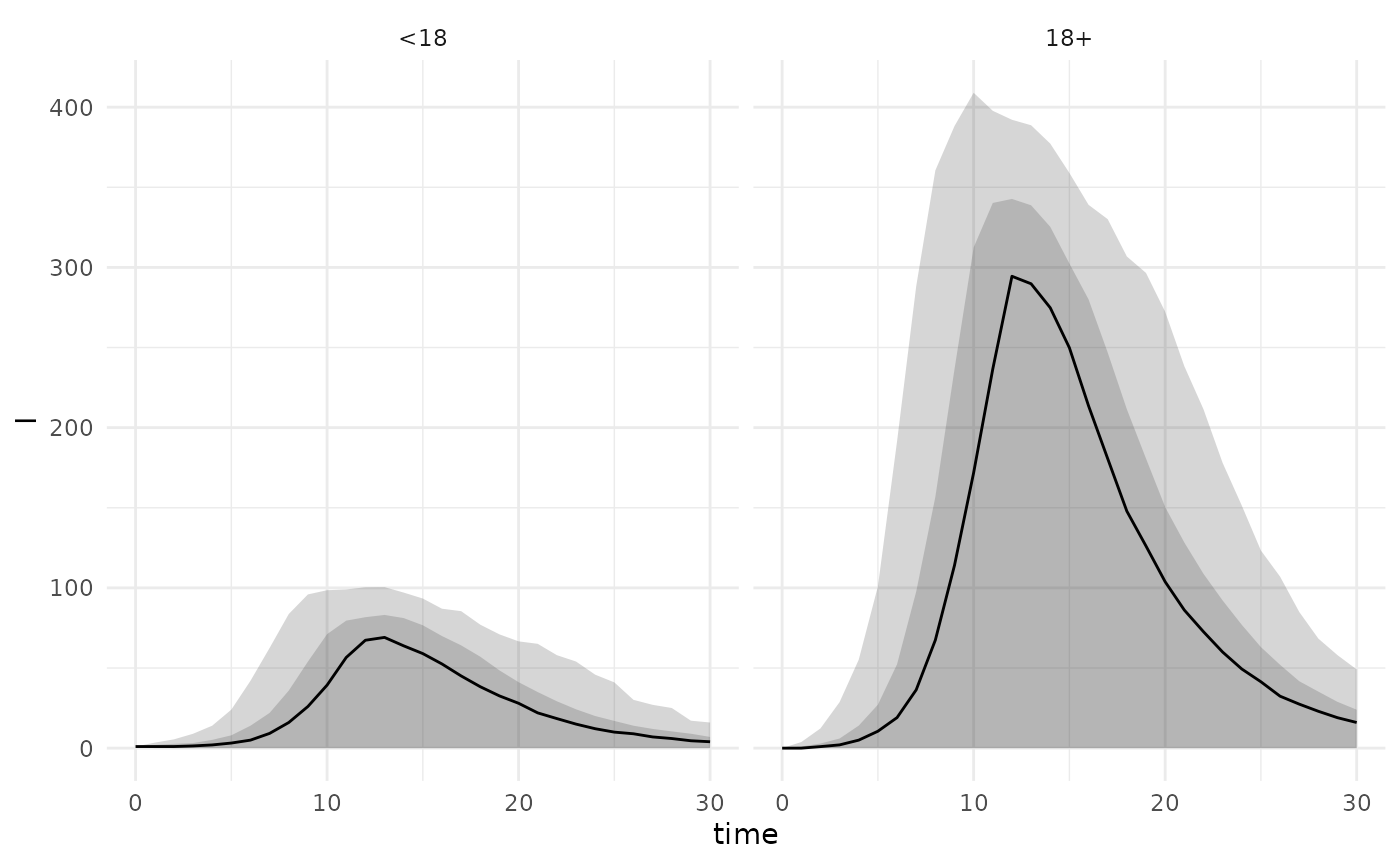
The final state can also be extracted by first making the projections longer and then examining the recovered individuals at the max time,
projections$projection |>
  create_age_group_column("R") |>
  filter(time == max(time)) |>
  ggplot(aes(fill=age_group,x=R)) +
  geom_density(alpha=0.2) +
  labs(x = "Final size",fill="")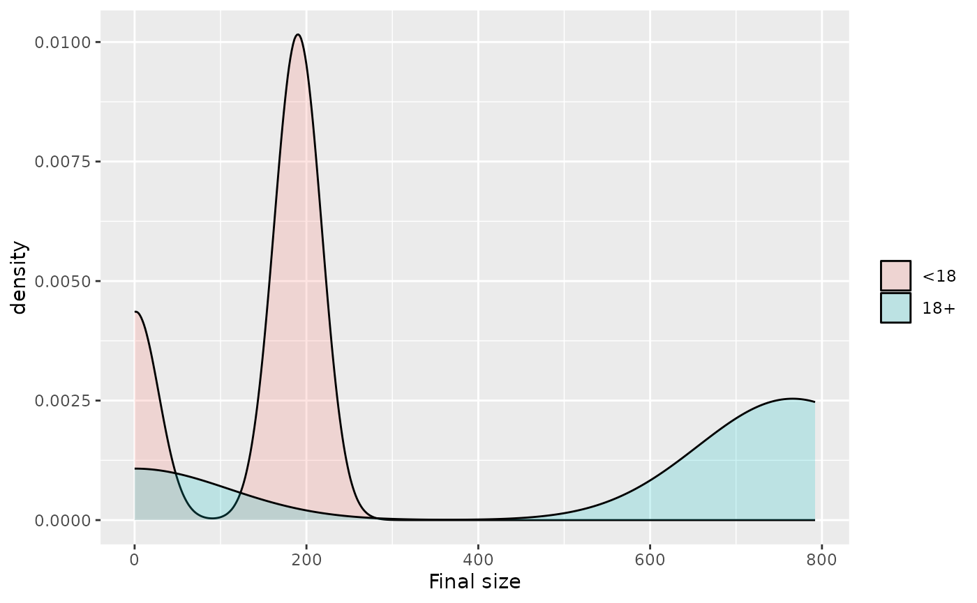
Fitting initial conditions
abc_stochastic_model can also take in initial states in
its fitting using the optional states argument. This needs
to be a complete model state for each row e.g.,
N <- c(200,800)
vaccine_rate <- c(0.1, 0.5)
infection_rate <- c(0.02,0.01)
nsamples <- 100
V <- matrix(rbinom(2*nsamples, size = rep(N, times = nsamples),
              prob = rep(vaccine_rate, times = nsamples)),
       nrow = nsamples, byrow = TRUE)
S <- matrix(rep(N,times=nsamples), nrow=nsamples,byrow = TRUE) - V
# simulation initial infections
I <- matrix(rbinom(2*nsamples, size = rep(N, times = nsamples),
              prob = rep(infection_rate, times = nsamples)),
       nrow = nsamples, byrow = TRUE)
zero_state <- matrix(rep(0,times=2*nsamples), nrow=nsamples)
states <- as.data.frame(cbind(S, V, I, zero_state))
colnames(states) <- c("S_<18", "S_18+", "V_<18", "V_18+",
                      "I_<18", "I_18+", "R_<18", "R_18+")
head(states)
#>   S_<18 S_18+ V_<18 V_18+ I_<18 I_18+ R_<18 R_18+
#> 1   188   412    12   388    12    10     0     0
#> 2   178   401    22   399     4     8     0     0
#> 3   183   384    17   416     3     8     0     0
#> 4   183   384    17   416     4     5     0     0
#> 5   184   376    16   424     5     2     0     0
#> 6   175   414    25   386     5     3     0     0
We can also project from a set of states with associated parameters
# fix beta parameter
sm <- sm |> update_parameters(beta = 0.1)

# define scenario based on list of states
example_scenario <- scenario_stochastic_model(sm, states = states)
state_projections <- projection_stochastic_model(example_scenario)
plot(state_projections, state = "I")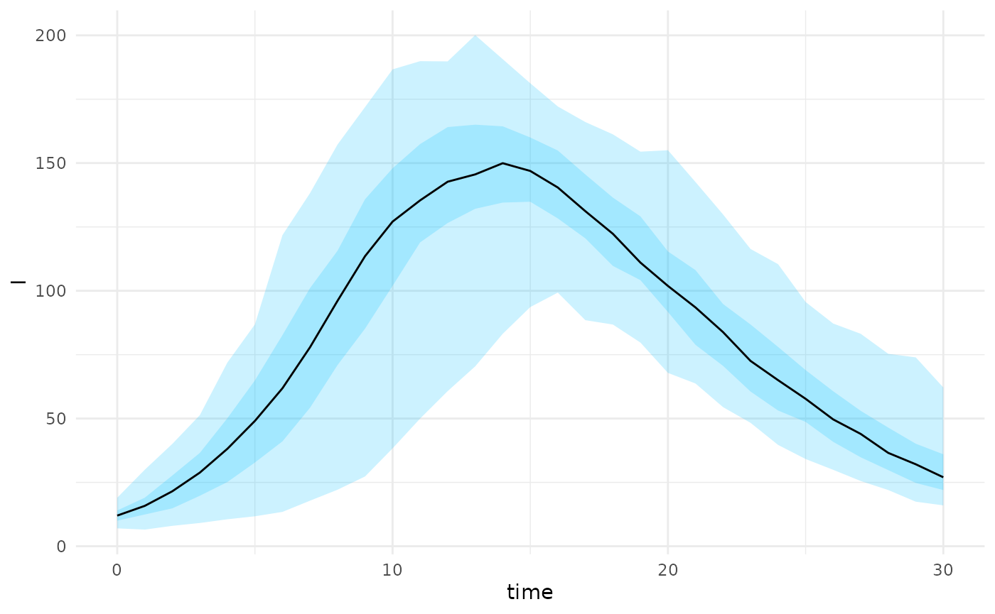
We can perform model fitting as before using the states
as a prior in the model that it is sampled from. In the example below we
generate some data with an initial distribution of vaccinated among
children and adults and use the number of recovered in each age group as
the summary function.
age_scenario <- list(
  params = list(beta = 0.1, gamma = 0.2, N = 1000),
  initial_states = list(
    S = c(190, 400),
    V = c(10, 400),
    I = c(1, 0),
    R = c(0, 0)
    ),
  sim_args = list(T = 10)
)

age_scenario <- age_scenario |>
  create_age_initial_conditions(age_groups)


sm <- stochastic_model(reactions,age_scenario)

r <- run_sim(sm) |> as.data.frame()

stat_func <- function(m){
  #' get total cases by age group
  m[nrow(m),startsWith(colnames(m),"R")]
}

cumulative_cases <- stat_func(r)
# simulate from prior
priors <- tibble("beta" = pmax(0,rnorm(100,mean=0.1,sd=0.1)))


res <- abc_stochastic_model(sm,priors,cumulative_cases,stat_func,
                            states = states)

plot(res, param = "beta")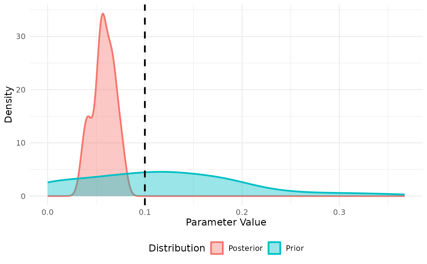
Using multisession and progressr
Both abc_stochastic_model and
projection_stochastic_model can be parallelized using the
future package together with progressr to
generate a progress bar. For more complex and realistic models these
will be essential to speed up computation and monitor progress. An
example of its use with two workers is provided below,
# set up multisession environment
plan(multisession, workers = 2)

# run projections in parallel
progressr::with_progress({
  state_projections <- projection_stochastic_model(example_scenario)
})